Variational Autoencoder (VAE)
What is VAE
A Variational Autoencoder models data by introducing a latent variable \(z\):
\[ p_\theta(x) = \int p_\theta(x|z)\, p(z)\, dz \]
- Decoder \(p_\theta(x|z)\): generates data from latent code (e.g., Gaussian with learned mean)
- Prior \(p(z) = \mathcal{N}(0, I)\): simple distribution over latent space
- Encoder \(q_\phi(z|x)\): approximate posterior (recognition network)
The marginal \(p_\theta(x)\) is intractable because the integral over \(z\) has no closed form.
How to Learn
Maximize the Evidence Lower Bound (ELBO) instead of the intractable log-likelihood:
\[ \log p_\theta(x) \geq \underbrace{\mathbb{E}_{q_\phi(z|x)}[\log p_\theta(x|z)]}_{\text{reconstruction}} - \underbrace{D_{\mathrm{KL}}(q_\phi(z|x) \| p(z))}_{\text{regularization}} \]
- Reconstruction term: decoder should reconstruct \(x\) from sampled \(z\)
- KL term: encoder posterior should stay close to the prior
- Use the reparameterization trick to backprop through sampling: \(z = \mu + \sigma \odot \epsilon\), where \(\epsilon \sim \mathcal{N}(0, I)\)
Intuition
- The encoder compresses data into a structured latent space
- The KL term prevents the latent space from degenerating (forces it to be smooth and continuous)
- At generation time, sample \(z \sim p(z)\) and decode — no encoder needed
- Trade-off: too strong KL → posterior collapse (latent ignored); too weak KL → poor generation
Examples
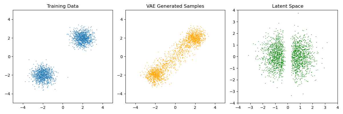
We use the same 2D Gaussian mixture to demonstrate VAE learning a generative model.
import torch
import torch.nn as nn
from torch.utils.data import DataLoader, TensorDataset

n = 2000
mix = torch.cat([
    torch.randn(n // 2, 2) * 0.5 + torch.tensor([2.0, 2.0]),
    torch.randn(n // 2, 2) * 0.5 + torch.tensor([-2.0, -2.0]),
])
dataloader = DataLoader(TensorDataset(mix), batch_size=128, shuffle=True)
class VAE(nn.Module):
    def __init__(self, data_dim=2, latent_dim=2, hidden=64):
        super().__init__()
        # Encoder: x -> (mu, log_var)
        self.encoder = nn.Sequential(
            nn.Linear(data_dim, hidden), nn.SiLU(),
            nn.Linear(hidden, hidden), nn.SiLU())
        self.fc_mu = nn.Linear(hidden, latent_dim)
        self.fc_logvar = nn.Linear(hidden, latent_dim)
        # Decoder: z -> x
        self.decoder = nn.Sequential(
            nn.Linear(latent_dim, hidden), nn.SiLU(),
            nn.Linear(hidden, hidden), nn.SiLU(),
            nn.Linear(hidden, data_dim))

    def encode(self, x):
        h = self.encoder(x)
        return self.fc_mu(h), self.fc_logvar(h)

    def reparameterize(self, mu, logvar):
        std = (0.5 * logvar).exp()
        return mu + std * torch.randn_like(std)

    def decode(self, z):
        return self.decoder(z)

    def forward(self, x):
        mu, logvar = self.encode(x)
        z = self.reparameterize(mu, logvar)
        return self.decode(z), mu, logvar
vae = VAE(data_dim=2, latent_dim=2, hidden=128)
opt = torch.optim.Adam(vae.parameters(), lr=1e-3)

n_epochs = 200
for epoch in range(n_epochs):
    # KL annealing: ramp beta from 0 to 0.1 over first 100 epochs
    beta = min(0.1, epoch / 1000.0)
    total_loss = 0.0
    for (x,) in dataloader:
        x_recon, mu, logvar = vae(x)
        recon_loss = ((x_recon - x) ** 2).sum(dim=1).mean()
        kl_loss = -0.5 * (1 + logvar - mu.pow(2) - logvar.exp()).sum(dim=1).mean()
        loss = recon_loss + beta * kl_loss
        opt.zero_grad()
        loss.backward()
        opt.step()
        total_loss += loss.item()
    if (epoch + 1) % 50 == 0:
        print(f"Epoch {epoch+1}: loss={total_loss / len(dataloader):.4f} beta={beta:.3f}")

# Generate samples from prior
with torch.no_grad():
    z_sample = torch.randn(500, 2)
    generated = vae.decode(z_sample)
print(f"Generated mean: {generated.mean(0).tolist()}")
print(f"Generated std:  {generated.std(0).tolist()}")
Visualize
Conclusion
The VAE successfully learns the bimodal structure:
- Generated samples match the two-cluster pattern of the training data, with correct centers (~(2,2) and ~(-2,-2)) and spread. However, there is noticeable density between the modes — this is the classic VAE "blurriness" caused by the Gaussian decoder averaging between modes.
- Latent space shows two separated clusters, confirming the encoder learned to map each data mode to a distinct latent region. The separation is clear but not as sharp as the data space — the KL regularization pulls both clusters toward the origin.
- Key trade-off: With low beta (0.1), the model preserves mode separation at the cost of a less regular latent space. With beta=1, the latent space would be smoother but generation would collapse to the mean between modes.
This illustrates a limitation of VAEs on multimodal data: the Gaussian prior + Gaussian decoder assumption makes it hard to produce zero density between modes. EBMs and diffusion models handle this better because they don't assume a simple parametric form for the output distribution.
References
- Kingma, D. P. & Welling, M. (2014). Auto-Encoding Variational Bayes. ICLR.
- Rezende, D. J., Mohamed, S., & Wierstra, D. (2014). Stochastic Backpropagation and Approximate Inference in Deep Generative Models. ICML.
- Sohn, K., Lee, H., & Yan, X. (2015). Learning Structured Output Representation using Deep Conditional Generative Models. NeurIPS.