EBM and Contrastive Learning
What is Energy-Based Model
Define a distribution via an unnormalized energy function \(E_\theta(x)\):
\[ p_\theta(x) = \frac{\exp(-E_\theta(x))}{Z_\theta}, \quad Z_\theta = \int \exp(-E_\theta(x))\, dx \]
- Low energy = high probability
- \(E_\theta\) can be any neural network (very flexible)
- The partition function \(Z_\theta\) is intractable — cannot compute or differentiate directly
How to Learn
The log-likelihood gradient decomposes into two terms:
\[ \nabla_\theta \log p_\theta(x) = -\nabla_\theta E_\theta(x) + \mathbb{E}_{x^- \sim p_\theta}\left[\nabla_\theta E_\theta(x^-)\right] \]
On the right hand side, the first term pushes energy down on real data and the second term pushes the energy up on model samples.
Contrastive Learning (Contrastive Divergence)
Approximate the intractable model expectation with short-run MCMC:
- Take data point \(x^+\)
- Initialize \(x^- = x^+\), run \(k\) steps of Langevin dynamics: \[ x^-_{t+1} = x^-_t - \frac{\eta}{2}\nabla_x E_\theta(x^-_t) + \sqrt{\eta}\,\xi_t \]
- Update parameters: \[ \theta \leftarrow \theta - \alpha\left[\nabla_\theta E_\theta(x^+) - \nabla_\theta E_\theta(x^-)\right] \]
This is CD-k (Contrastive Divergence). Biased but effective.
Intuition
- We want the real data to have lower energy (more probable).
- We want negative samples from short MCMC to have higher energy (less probable).
- The model learns a "landscape" where data sits in valleys
- If we replace x with τ, we will see inverse RL is 'contrastive learning' where negative samples come from trajectory optimization/RL rather than Langevin dynamics.
Example
We will use a simple example to demonstrate how it works. In this example, we draw data from a 2D mixture of two Gaussians:
- Cluster 1: n/2 points centered at (2, 2) with std dev 0.5 in each dimension
- Cluster 2: n/2 points centered at (-2, -2) with std dev 0.5 in each dimension
import torch
import torch.nn as nn
from torch.utils.data import DataLoader, TensorDataset
# --- Test Data: 2D Gaussian Mixture ---
n = 2000
mix = torch.cat([
    torch.randn(n // 2, 2) * 0.5 + torch.tensor([2.0, 2.0]),
    torch.randn(n // 2, 2) * 0.5 + torch.tensor([-2.0, -2.0]),
])
dataloader = DataLoader(TensorDataset(mix), batch_size=128, shuffle=True)
We model the energy function with a MLP and define langevin dynamics for sampling negative data:
# langevin dynamics for generating negative samples
def langevin_negative(ebm, x_init, steps=20, step_size=0.01):
    x = x_init.clone().detach().requires_grad_(True)
    for _ in range(steps):
        e = ebm.energy(x).sum()
        score = torch.autograd.grad(- e, x)[0]
        x = x.detach() + (step_size / 2) * score + (step_size**0.5) * torch.randn_like(x)
        x.requires_grad_(True)

    return x.detach()

# --- Model ---
class EBM(nn.Module):
    def __init__(self, dim=2, hidden=64):
        super().__init__()
        self.net = nn.Sequential(
            nn.Linear(dim, hidden), nn.SiLU(),
            nn.Linear(hidden, hidden), nn.SiLU(),
            nn.Linear(hidden, 1))

    def energy(self, x):
        return self.net(x).squeeze(-1)
# --- Training ---
ebm = EBM()
opt = torch.optim.Adam(ebm.parameters(), lr=1e-3)

for epoch in range(5):
    total_loss = 0.0
    for (x_pos,) in dataloader:
        x_neg = langevin_negative(ebm, x_pos, steps=20)
        loss = ebm.energy(x_pos).mean() - ebm.energy(x_neg).mean()
        opt.zero_grad()
        loss.backward()
        opt.step()
        total_loss += loss.item()
    print(f"Epoch {epoch}: loss={total_loss / len(dataloader):.4f}")

# --- Verify: energy should be lower on data than on random noise ---
noise = torch.randn(100, 2) * 3
data_sample = mix[:100]
print(f"Energy on data:  {ebm.energy(data_sample).mean().item():.4f}")
print(f"Energy on noise: {ebm.energy(noise).mean().item():.4f}")
Epoch 0: loss=-0.0094
Epoch 1: loss=-0.0248
Epoch 2: loss=-0.0492
Epoch 3: loss=-0.0763
Epoch 4: loss=-0.0918
Energy on data:  0.6611
Energy on noise: 6.8638
Visualize
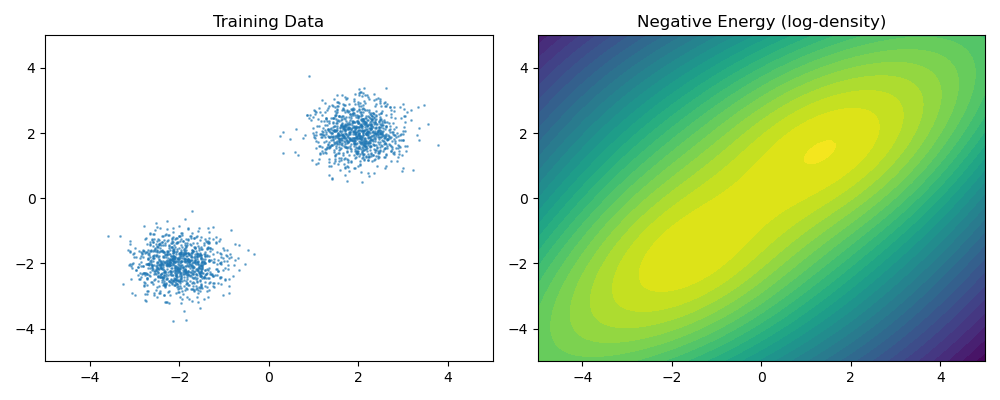
Training Animation (GIF)
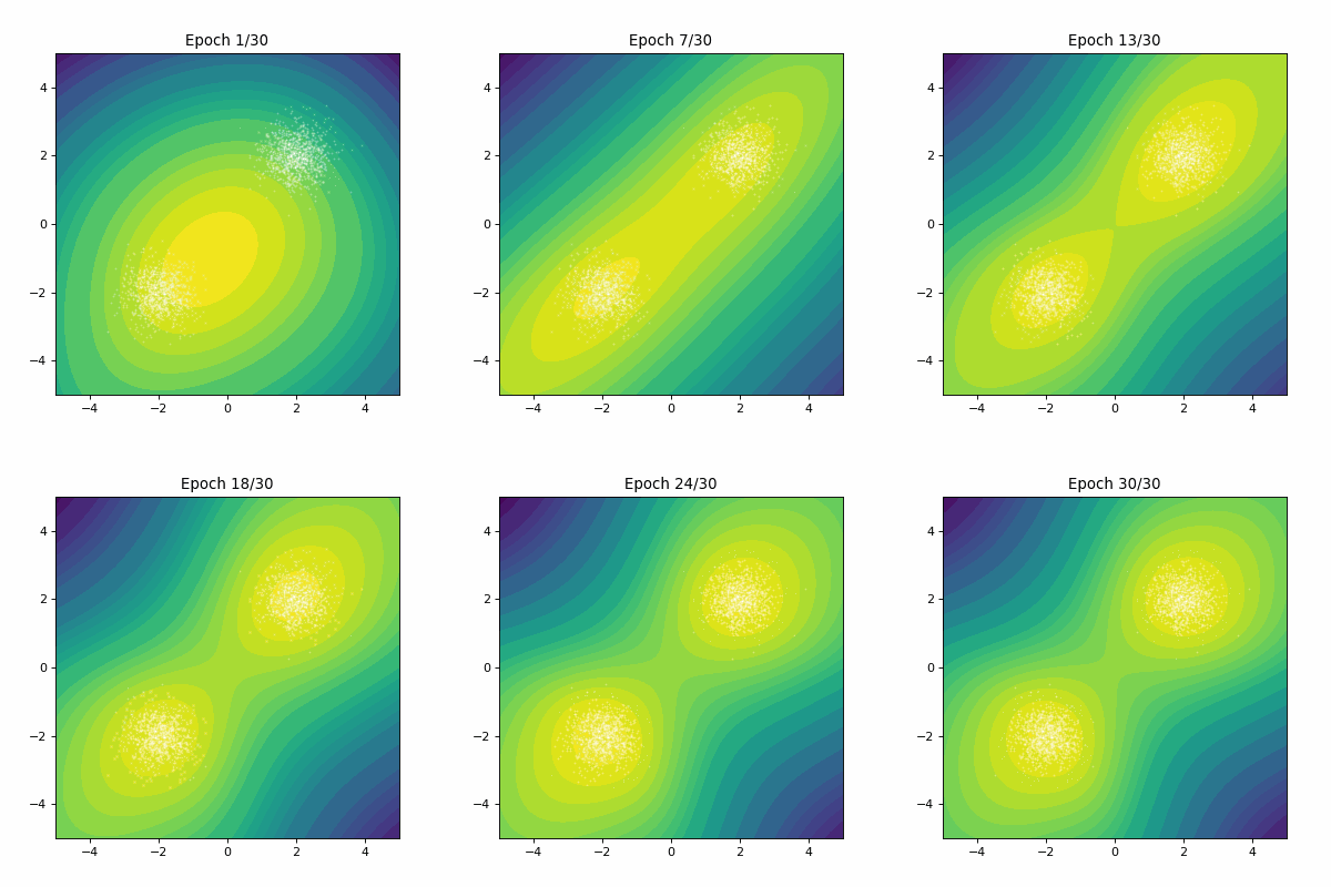
As we can see, the neural energy function learns to approximate the negative log-density of the data distribution, assigning lower energy to high-density regions.
References
- Hinton, G. (2002). Training Products of Experts by Minimizing Contrastive Divergence. Neural Computation.
- LeCun, Y., Chopra, S., Hadsell, R., Ranzato, M., & Huang, F. (2006). A Tutorial on Energy-Based Learning. In Predicting Structured Data.
- Du, Y. & Mordatch, I. (2019). Implicit Generation and Modeling with Energy-Based Models. NeurIPS.
- Grathwohl, W., Wang, K.-C., Jacobsen, J.-H., Duvenaud, D., Norouzi, M., & Swersky, K. (2020). Your Classifier is Secretly an Energy Based Model and You Should Treat it Like One. ICLR.
- Song, Y. & Ermon, S. (2019). Generative Modeling by Estimating Gradients of the Data Distribution. NeurIPS.