Flow matching
What is Flow Matching
Learn a time-dependent velocity field \(v_\theta(x, t)\) that transports a simple prior \(p_0 = \mathcal{N}(0, I)\) to the data distribution \(p_1 = p_{\text{data}}\) along straight paths:
\[ \frac{dx}{dt} = v_\theta(x, t), \quad t \in [0, 1] \]
- At \(t=0\): noise. At \(t=1\): data.
- The flow defines a deterministic mapping between noise and data (no stochasticity at inference)
- Unlike diffusion models, the paths are straight (optimal transport), making sampling fast
The key idea: define a conditional flow path between each noise-data pair as a linear interpolation:
\[ x_t = (1 - t)\, x_0 + t\, x_1, \quad x_0 \sim \mathcal{N}(0, I),\; x_1 \sim p_{\text{data}} \]
The conditional velocity along this path is simply \(v(x_t, t | x_0, x_1) = x_1 - x_0\).
How to Learn
Train a neural network to predict the conditional velocity field:
\[ \mathcal{L}(\theta) = \mathbb{E}_{t \sim U[0,1],\, x_0 \sim p_0,\, x_1 \sim p_1} \left[ \| v_\theta(x_t, t) - (x_1 - x_0) \|^2 \right] \]
Training procedure:
- Sample \(x_1 \sim p_{\text{data}}\) and \(x_0 \sim \mathcal{N}(0, I)\)
- Sample \(t \sim U[0, 1]\)
- Compute \(x_t = (1-t) x_0 + t\, x_1\)
- Regress \(v_\theta(x_t, t)\) toward target \(x_1 - x_0\)
Intuition
- No MCMC, no ELBO, no adversarial training — just regression
- The model learns "which direction to push" at each point and time
- At inference: start from noise, integrate the ODE forward with Euler steps
- Straight paths = fewer integration steps needed (vs. curved diffusion paths)
Examples
We use the same 2D Gaussian mixture to demonstrate flow matching.
import torch
import torch.nn as nn
from torch.utils.data import DataLoader, TensorDataset

n = 2000
mix = torch.cat([
    torch.randn(n // 2, 2) * 0.5 + torch.tensor([2.0, 2.0]),
    torch.randn(n // 2, 2) * 0.5 + torch.tensor([-2.0, -2.0]),
])
dataloader = DataLoader(TensorDataset(mix), batch_size=128, shuffle=True)
class VelocityNet(nn.Module):
    def __init__(self, data_dim=2, hidden=128):
        super().__init__()
        # Input: x (2D) + t (1D) = 3D
        self.net = nn.Sequential(
            nn.Linear(data_dim + 1, hidden), nn.SiLU(),
            nn.Linear(hidden, hidden), nn.SiLU(),
            nn.Linear(hidden, data_dim))

    def forward(self, x, t):
        # t: (batch,) -> (batch, 1)
        return self.net(torch.cat([x, t.unsqueeze(-1)], dim=-1))
model = VelocityNet()
opt = torch.optim.Adam(model.parameters(), lr=1e-3)

for epoch in range(200):
    total_loss = 0.0
    for (x1,) in dataloader:
        x0 = torch.randn_like(x1)           # noise
        t = torch.rand(x1.shape[0])          # random time
        xt = (1 - t.unsqueeze(1)) * x0 + t.unsqueeze(1) * x1  # interpolate
        target = x1 - x0                     # conditional velocity
        pred = model(xt, t)
        loss = ((pred - target) ** 2).sum(dim=1).mean()
        opt.zero_grad()
        loss.backward()
        opt.step()
        total_loss += loss.item()
    if (epoch + 1) % 50 == 0:
        print(f"Epoch {epoch+1}: loss={total_loss / len(dataloader):.4f}")
Generate Samples (ODE Integration)
@torch.no_grad()
def sample_ode(model, n_samples=2000, steps=50):
    x = torch.randn(n_samples, 2)
    dt = 1.0 / steps
    for i in range(steps):
        t = torch.full((n_samples,), i * dt)
        x = x + model(x, t) * dt
    return x

samples = sample_ode(model)
print(f"Sample mean: {samples.mean(0).tolist()}")
print(f"Sample std:  {samples.std(0).tolist()}")
Visualize
Conclusion
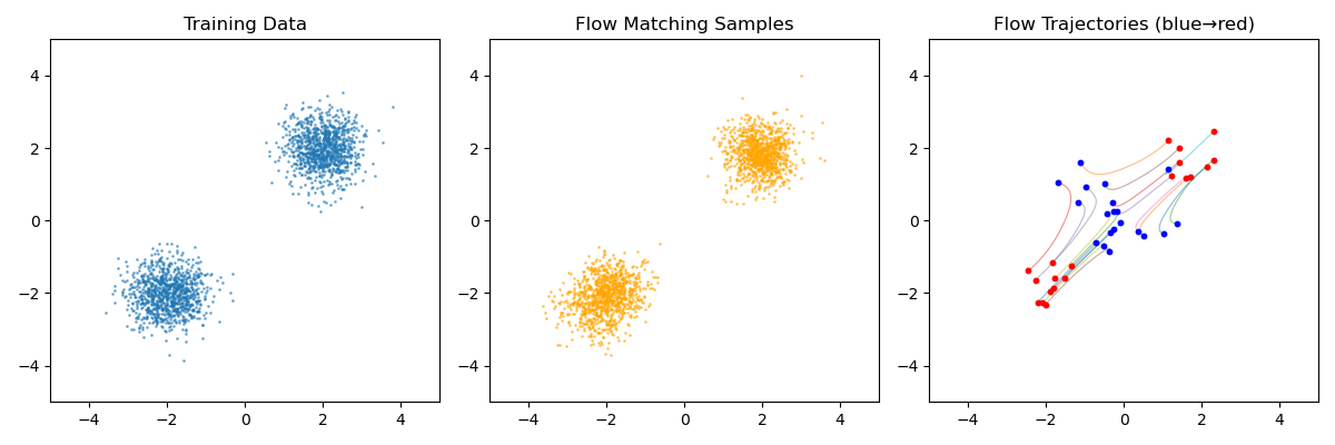
Flow matching produces sharp, well-separated bimodal samples with no inter-mode leakage:
- Sample quality: The generated samples closely match the training data — two tight clusters at the correct locations with no spurious density between modes. This is a clear improvement over VAE which produced a "bridge" of samples between clusters.
- Non-straight trajectories: Although training uses linear interpolation (straight conditional paths per noise-data pair), the learned marginal velocity field produces curved trajectories at inference. This is because the network predicts an averaged velocity over all possible pairings at each location — early in the flow, the velocity is a mixture of directions toward both modes, and the path curves as it commits to one.
- Mode assignment: The trajectories show that noise points are routed to the nearest mode — points starting in the upper-right flow to (2,2), points starting lower-left flow to (-2,-2). The velocity field learns a clean partition of space.
- Comparison to other methods:
- vs. EBM: No MCMC needed at inference — just deterministic ODE integration
- vs. VAE: No blurriness or inter-mode leakage — the deterministic flow avoids the Gaussian decoder averaging problem
- vs. Diffusion: Simpler training objective (regression vs. score matching); fewer integration steps needed in practice (50 here vs. 1000 typical for DDPM)
References
- Lipman, Y., Chen, R. T. Q., Ben-Hamu, H., Nickel, M., & Le, M. (2023). Flow Matching for Generative Modeling. ICLR.
- Liu, X., Gong, C., & Liu, Q. (2023). Flow Straight and Fast: Learning to Generate and Transfer Data with Rectified Flow. ICLR.
- Tong, A., Malkin, N., Huguet, G., Zhang, Y., Rector-Brooks, J., Fatras, K., Wolf, G., & Bengio, Y. (2024). Improving and Generalizing Flow-Based Generative Models with Minibatch Optimal Transport. TMLR.